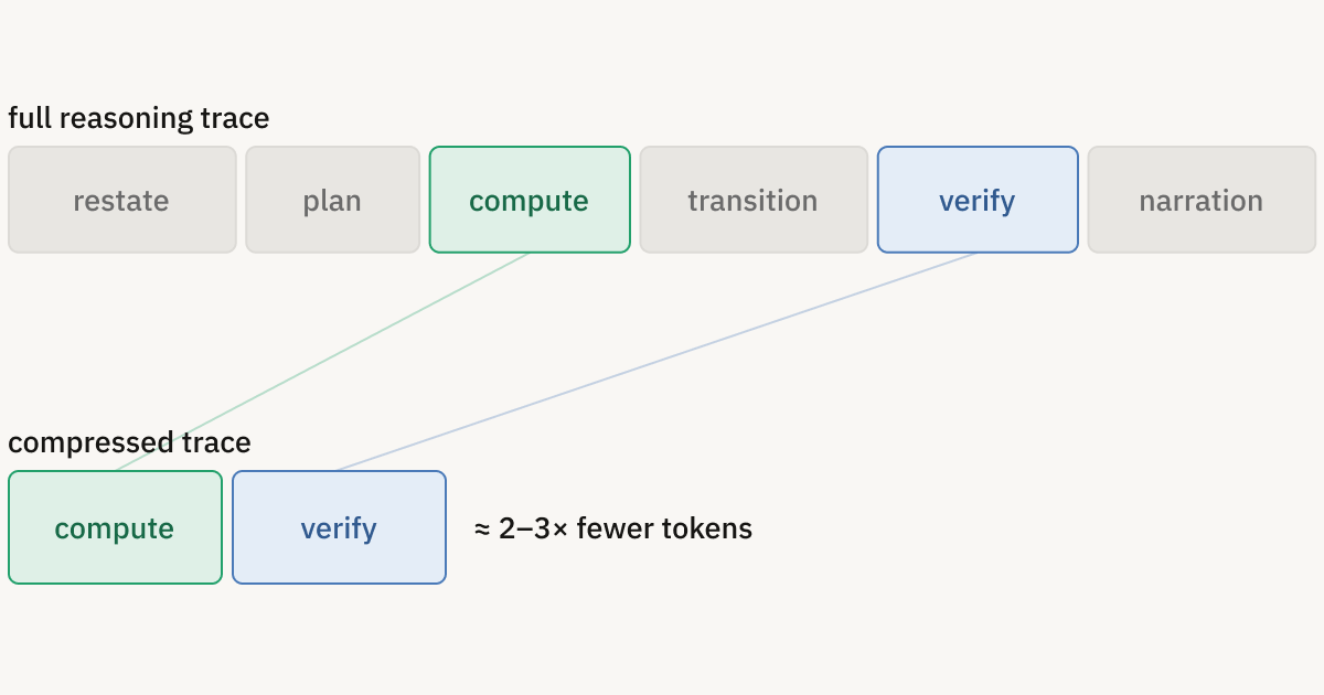
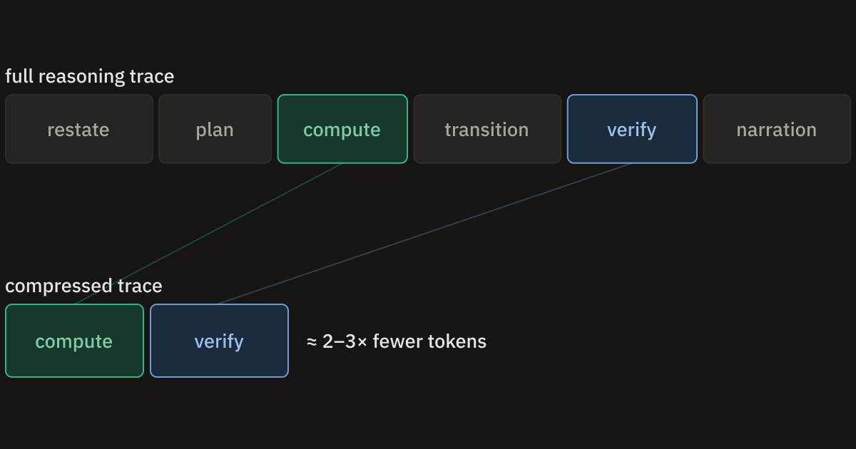
Reasoning models are natural over-thinkers: they can spend hundreds of tokens answering to a simple ”Hello!”; they love to restate the given problems, to narrate all of their transitions, and it doesn’t happen rarely that the tokens needed for the actual computation are just a fraction of those that get generated. It comes naturally to the mind that if we could compress this reasoning, dropping the fluff, the restatements and the narration, we would get the same answers faster. But is this intuition provably correct? Or are we being too naive?
Spoiler: it works! But let’s analyze things step by step.
Reasoning compression
Reasoning (and output) compression is not a new science: “caveman”-prompting 1A technique consisting in prompting an LLM to drop articles, fillers ('just', 'really', 'basically', etc.), pleasantries, and to prefer short synonyms. 1A technique consisting in prompting an LLM to drop articles, fillers ('just', 'really', 'basically', etc.), pleasantries, and to prefer short synonyms. for output compression has been around for a while now, and models trained specifically with caveman-compressed traces are starting to come out already. Multiple reasoning leaks from GPT-5.5 also suggest that OpenAI took that same approach to optimize the token efficiency of their latest frontier LLMs.
With these premises, I decided to start working on Flint (Flint as in “The Flint-stones”), a project originally comprised of a dataset of caveman-compressed reasoning traces (with the post-thought answers kept verbatim) and a series of models fine-tuned on this dataset. Things did not go well from the start, let’s see why.
So, what went wrong?
The original flint-sft dataset pipeline was the following:
- Get real reasoning traces from gemma-4-31B-it
- Compress the whole traces (foreshadowing) using fast, online, free LLMs (at the time stepfun-ai/Step-3.7-Flash and nvidia/NVIDIA-Nemotron-3-Ultra-550B-A55B were available for free on the Nous Portal)
Gemma was chosen as the most praised open LLM for reasoning efficiency (both by the community and by reputable benchmarks), and I was self-convinced that the compressor model would not matter as long as the instructions (how to compress) were followed nicely; though, it seems like I was wrong!
Because of GPU constraints, I decided to train gemma-4-12B-it instead of the 31B release from which I took the traces, and results were… horrible! I did not record the data (at the time I just thought I would leave the project there, without touching it ever again, “R.I.P. Flint”), though from what I remember looping had increased significantly, and performance in the AIME2026 benchmark got ~halved.
Why did this happen? Well, let’s start with two (now very obvious) problems in this old pipeline of mine:
- The model was tuned on traces generated from another model.
- The traces were compressed using yet another model.
Both of these say the same thing: the distributions 2The numerical scores for each token at each step, considering the entire tokens sequence. 2The numerical scores for each token at each step, considering the entire tokens sequence. of the original model were different from both the traces generator and the compressor.
Isn’t distillation from bigger to smaller models a proven strategy?
If you are into the more technical side of the LLMs world, you may know that: yes, training smaller models on the outputs of bigger models is a very well proven technique to efficiently improve the small models performance (and the big labs are wary of that), but we need to add a few important notes:
- Distillation prefers full logits distributions: usually we record the scores for each token for each step and use that distributions in training, while for Flint only the chosen token at each step was used for training (that’s a lot less data per step).
- Distillation generally needs a lot of data, and the more it has to skew the original model distribution the more data will be needed: my original dataset, while “biggish” (15k examples, a lot more than the final, and successful, datasets), is not nearly big enough to skew the distribution of the original model in a good way given the initial distance between them.
So yes, distillation is a good and proven strategy, but only if done right.
The new pipeline
Before starting to experiment again on Flint, I decided to completely redo the data pipeline. With the new intuition in hand (“self-distillation may solve all of my problems!“) I decided to create crucible, a merged dataset with over 37k rows that combines logical, creative and multilingual task types, specifically designed with distillation in mind.
The idea now changed to the following: take crucible and an LLM we want to optimize, generate samples from crucible with that LLM (produces a crucible-sft-model_name dataset), compress the traces (produces a flint-sft-model_name dataset), and tune the original LLM on the compressed traces (produces a model_name-flint model).
New pipeline, new problems
I decided to test the new pipeline on a small model first, Qwen/Qwen3.5-4B, and that’s when I found another hard stop. While the control I created worked perfectly fine now (crucible-sft-model_name, the uncompressed SFT dataset, was used to tune the original LLM and showed no performance degradation), the (flat, “whole trace”) compression-trained model showed signs of collapse with greedy decoding (temperature=0 3Temperature is an inference-time value settable between 0 and 2 (by convention, the upper limit is not strict) that controls creativity (or even better, the *unpredictability* of the outputs). Setting temperature to 0 generally means that we are doing deterministic generation, so re-running a generation at temperature=0 shall always return the same answer. 3Temperature is an inference-time value settable between 0 and 2 (by convention, the upper limit is not strict) that controls creativity (or even better, the *unpredictability* of the outputs). Setting temperature to 0 generally means that we are doing deterministic generation, so re-running a generation at temperature=0 shall always return the same answer.): lots of doom loops, degraded performance.
| Benchmark | accuracy | avg reasoning tokens | loop rate | truncation rate |
|---|---|---|---|---|
| GSM8K | .03 | 7,960 | .93 | .97 |
| MATH-500 | .02 | 8,033 | .64 | .98 |
| HumanEval | .04 | 7,919 | .55 | .96 |
| MBPP | .01 | 8,019 | .84 | .97 |
| MMLU-Pro | .05 | 7,499 | .42 | .90 |
Now, a result that really surprised me… At temperature=1, the model was fine, more than fine actually; let’s look at the temperature sweep benchmark:
| GSM8K loop sweep @ t=0 (n=50) | Accuracy | Loop rate | Avg reasoning tokens | Truncated rate |
|---|---|---|---|---|
| original model | .64 | .28 | 3915.1 | .36 |
| uncompressed SFT | .54 | .34 | 4894.2 | .44 |
| flat compression | .02 | .96 | 8030.5 | .98 |
| GSM8K loop sweep @ t=0.6 (n=50) | Accuracy | Loop rate | Avg reasoning tokens | Truncated rate |
|---|---|---|---|---|
| original model | .68 | .12 | 3827.4 | .32 |
| uncompressed SFT | .58 | .22 | 4729.8 | .42 |
| flat compression | .20 | .74 | 6531.3 | .78 |
| GSM8K loop sweep @ t=1 (n=50) | Accuracy | Loop rate | Avg reasoning tokens | Truncated rate |
|---|---|---|---|---|
| original model | .74 | .00 | 4140.6 | .26 |
| uncompressed SFT | .64 | .18 | 4319.3 | .36 |
| flat compression | .90 | .04 | 1500.9 | .06 |
Note: “GSM8K loop sweep” is a small random (fixed) subset of GSM8K we used for our fast temperature sweep benchmarks.
Setting the temperature=1 made the model incredibly good, both in accuracy and in token usage (+16 points and less than half the tokens!!); so, how and why did greedy decoding break? First, something you should know: reasoning models usually perform better at higher temperatures; you can see this in the results for the original model, and also on the models’ own pages (Qwen itself suggests a temperature between 0.6 and 1.0).
A higher temperature helps the model escape loops: “Wait, let me try this instead…” and similar phrases are often used by reasoning LLMs to move out of a failed attempt, but these same phrases are also the same on which they can easily get stuck. A higher temperature here helps by flattening the probabilities of our tokens, making the re-use of the exact phrases less probable.
Our loops, though, are kind of special:
.
.
.
.
.
.
Correct.
[… repeats identically, hundreds of times]
What’s interesting here is that 623 was actually the right answer; the model did not loop in an intermediate verification step. So, the thinking did not really break, but what broke is the stopping mechanism. We will come back to this later, when we better analyze loops and recent proposed solutions. Now let’s move to the headline experiment!
Section-aware compression
What if we compress (or drop) only the non-computation spans of our traces? Let me explain: in the introduction we talked about how LLMs are especially inefficient in everything that is not “raw computation” (as in, useful reasoning to solve a problem, step-by-step calculations etc.), so the new idea is: keep the computation verbatim (and the verification steps too), and compress or drop the remaining sections (restatements, planning, transitions, narration).
This adds a step in our data pipeline: we now need an LLM to take the traces and to label each section for us before compression happens; but the results, let me assure you, are well worth the effort. Look at the chart and table below to get an idea:
| GSM8K t=0 | accuracy | avg reasoning tokens | loop rate |
|---|---|---|---|
| original model | .575 | 4,413 | .22 |
| uncompressed SFT | .62 | 4,402 | .25 |
| flat compression | .03 | 7,960 | .93 |
| section-aware | .77 | 2,586 | .11 |
| section-aware, trained bare | .82 | 1,524 | .12 |
I am also throwing in the temperature sweep data:
| GSM8K loop sweep @ t=0 (n=50) | accuracy | avg reasoning tokens | loop rate |
|---|---|---|---|
| original model | .64 | 3,915 | .28 |
| uncompressed SFT | .54 | 4,894 | .34 |
| flat compression | .02 | 8,031 | .96 |
| section-aware | .82 | 2,211 | .14 |
| section-aware, trained bare | .86 | 1,228 | .10 |
| GSM8K loop sweep @ t=0.6 (n=50) | accuracy | avg reasoning tokens | loop rate |
|---|---|---|---|
| original model | .68 | 3,827 | .12 |
| uncompressed SFT | .58 | 4,730 | .22 |
| flat compression | .20 | 6,531 | .74 |
| section-aware | .84 | 2,266 | .08 |
| section-aware, trained bare | .82 | 1,911 | .12 |
| GSM8K loop sweep @ t=1 (n=50) | accuracy | avg reasoning tokens | loop rate |
|---|---|---|---|
| original model | .74 | 4,141 | .00 |
| uncompressed SFT | .64 | 4,319 | .18 |
| flat compression | .90 | 1,501 | .04 |
| section-aware | .78 | 2,610 | .08 |
| section-aware, trained bare | .74 | 3,373 | .16 |
Notice the “trained bare” addition, we will get back to it soon.
As you can observe, section-aware training completely solves the greedy collapse, and beats not only the collapsed compression-trained model, but also the original model and our control, while using about a third of the tokens in the bare trained variant! Flat compression still dominates in the temperature=1 benchmark, but section-aware is still satisfactory, achieving the same score as the original model while using ~19% less tokens, and it also remains stable at lower temperatures; keep in mind that only 50 samples are present in the loop sweep benchmark. Also notice how for the section-aware model the number of doom loops increased together with the temperature.
Training bare
For this study I ran many compression experiments; the more questions came up the more experiments needed to be run. At one point one of my questions was: does training with a system prompt affect performance? Initially we decided to use a system prompt (e.g. “Please reason step by step, and put your final answer within \boxed{}.” for the math domain), but what I found is that not including the system prompt at training time, and only including it at eval time, improves performance significantly!
Check the full bench sweep for the 2 models below:
| trained WITH prompt | accuracy | avg reasoning tokens | loop rate | truncation rate |
|---|---|---|---|---|
| GSM8K | .77 | 2,586 | .11 | .22 |
| MATH-500 | .53 | 5,120 | .16 | .47 |
| HumanEval | .53 | 5,047 | .16 | .43 |
| MBPP | .41 | 6,090 | .32 | .59 |
| MMLU-Pro | .52 | 4,427 | .14 | .35 |
| trained W/O prompt | accuracy | avg reasoning tokens | loop rate | truncation rate |
|---|---|---|---|---|
| GSM8K | .82 | 1,524 | .12 | .15 |
| MATH-500 | .57 | 3,821 | .25 | .43 |
| HumanEval | TBD | — | — | — |
| MBPP | TBD | — | — | — |
| MMLU-Pro | TBD | — | — | — |
Training without a prompt gives us better performance with less tokens at inference time, but why is that? My hypothesis here is behavior gating: using system prompts while training on a new behavior makes that behavior be gated behind the used prompts; while you may think that under this assumption the prompt-trained model shall perform just like the bare-trained one given that the system prompt is available at inference time, it is possible that by training without the system prompts the per-domain gains accumulated, while training with the prompts may have caused the gains to be split in domain-side compartments.
To verify a form of behavior gating I also decided to train the model with and without an identity system prompt; this prompt tells the model everything about the style it shall follow, how to speak and so on. The result was positive and training the model with this identity prompt effectively gates the compressed reasoning behavior behind it: if you use this system prompt at eval time the reasoning is compressed, otherwise it is not and the model performs just like the original.
Can we fix the greedy collapse?
Just around the time I started re-experimenting on Flint, a new research post by Liquid AI was released: Reducing Doom Loops with Final Token Preference Optimization. This post illustrates a new technique designed to kill doom loops: “oh, couldn’t that be exactly we need to fix the flat compression collapse under greedy decoding?” that’s what I thought, but the answer was a solid no.
Remember when we talked about the loops we got before, and about how they were special. Antidoom works by making the loop-causing tokens less probable in the output distribution of a model, but that our flat compression models loop on tokens that we should absolutely not remove: they often loop on numbers, sometimes even on the final answer; we can’t make number and the correct solution LESS probable! Or maybe, we can: I actually ran FTPO, against my own intution, and following are the results:
| Arm | accuracy | avg reasoning tokens | loop rate | truncation rate |
|---|---|---|---|---|
| sft-flint-adaptive-v2 | .03 | 7,960 | .93 | .97 |
| sft-flint-adaptive-v2-antidoom | .00 | 8,192 | .81 | 1.00 |
Long story short: the loops do decrease, but the model is not able to ever find or output the answer; even when it does not loop it can’t stop trying to output a solution it will never be able to output. Sounds like a nightmare to me, so let’s stop experimenting with antidoom here, just to be safe in case LLMs ever become sentient.
What else did not work?
I also wanted to share a few more failed intuitions I got while working on Flint (after all, sharing failures is also important to accelerate research):
- “If we keep the last section of the reasoning trace verbatim, the model may stop looping.” Nope: the flat compression model still collapses into loops even when retaining the original trace’s closure.
- “Training for more epochs may improve things” No again: I tried training with flat compression for 3 epochs instead of 2 but the result was just a worse model overall, both in accuracy and length of the reasoning.
- “I shall try using a better model as the segmenter for section-aware training.” That also did not work; why? I don’t have a definitive answer yet. I tested training with segmentation done by a bigger LLM while still delegating the compression step to the original model, but the result was, once again, a worse model overall.
What about non-reasoning tasks?
I built crucible with the objective to also retain writing abilities: included are multilingual, open-ended, creative queries. These are (obviously) not objectively verifiable, but we used an LLM-as-a-judge to compare the samples from our compressed models against those generated by the original model, and the (section-aware, the only we tested) compressed models won more overall, while using around 10% less thinking tokens; even though this does not mean that the compressed models write better, we can assume that they at least don’t write much worse.
Do all of these findings transfer across families and sizes?
When I decided I was satisfied with the results I got with Qwen3.5-4B, I decided to move on to gemma-4-12b-it; we are changing model family (in particular, the underlying architecture) and size. As I was resource constrained at this point (distilling and tuning a 12b model at home takes time) I decided to only train the uncompressed SFT control and a compressed variant with the best settings we got so far: a section-aware, bare trained version.
So, how did it go? The answer is: surprisingly well! Check the table below:
| gemma-4-12b | GSM8K | MATH-500 | HumanEval |
|---|---|---|---|
| original model | .57 @ 3,753 (41% trunc) | .51 @ 5,078 | .31 @ 6,107 (69% trunc) |
| uncompressed SFT (control) | .68 @ 2,942 (30% trunc) | .60 @ 4,231 | — |
| section-aware, trained bare | .86 @ 1,679 (10% trunc) | .49 @ 4,883 | .57 @ 4,777 (43% trunc) |
The compressed model performs a lot better already, both in math and in code generation. But, how does reasoning in a compressed style improve accuracy? We also noticed this with qwen, so, why is happening? Did the model get distracted by the many useless tokens it generated? Maybe it is because using less tokens the context does not get too big and context degradation is less pronounced? Those are real possibilities, but the most obvious answer here is… the original model just thinks for too much time, so much so that it’s results got truncated 41% of the times in GSM8K.
That is also the reason why our control also performs better than the original model; the uncompressed traces we used are verified, so only those that actually get to a right answer got included in the training, and that alone steered the behavior of gemma in a good way. gemma-12b might just not be a well optimized reasoner from the start, and for this reason we are able to get massive improvements here.
Temperature sweep surprises
Remember how our section-aware trained Qwen got worse at higher temperatures while being a beast at temperature=0? Well, surprisingly, compressed gemma is also a beast at higher temperatures, and it actually gets better the higher the temperature gets!
This means that compressed gemma is retaining the temperature behavior of its original weights, and that this model I built is overall better; I honestly wasn’t satisfied with the results I got from Qwen: either a better model at temperature=0 but mid at higher temps or a better model at temperature=1 but worse at lower temps. This compressed gemma is what I hoped to get from the start, and that is why I also released it on Hugging Face, as a merged checkpoint!
Takeaways
To conclude, what did we learn today?
- Termination is the number one failure we had to deal with, so be aware of it if you’d also try to play with an LLM’s brain in the future.
- A behavior can be easily gated, and this is honestly pretty cool; imagine training a same model with different system prompts to enable or disable various capabilities at will, all in the same weights. I’ll personally experiment more on that in the near future.
- Distilling across models is more complex than it sounds like; also keep this in mind the next time you see a “Opus-Fable-GPT-MaximumPerformance-BESTMODELEVER” tune on Hugging Face, they are probably worse than the original models anyway.
Artifacts
I have also published all the artifacts that got generated in this study (LoRA adapters and datasets), together with a full logbook and code; I’ll leave you to them!
- caveman-reasoning-compression (Hugging Face)
- reasoning-compression-ablation-arms (Hugging Face)
- marcodsn/reasoning-compression (GitHub)
The code and the logbook were produced by an agent (Fable); the ideas, chosen experiments, successful and failed intuitions are mine.
Citation
Please cite this work as:
De Santis, Marco, "Compressing Reasoning Without Breaking It", marcodsn.me, Jul 2026.
Or use the BibTeX citation:
@misc{desantis2026reasoningcompression,
  author = {Marco De Santis},
  title = {Compressing Reasoning Without Breaking It},
  year = {2026},
  month = jul,
  url = {https://marcodsn.me/blog/reasoning-compression}
}